Duplication rate
RustQC reimplements seven tools from the RSeQC package. Each tool produces output files that match the format and content of the original Python implementation, plus native PNG and SVG plots generated directly — no R scripts required.
All RSeQC tools run automatically as part of the rustqc rna command and use
the input filename stem as a prefix for output files. Output files are organized
into per-tool subdirectories under rseqc/. For example,
rustqc rna sample.bam --gtf genes.gtf -o results/ produces
RSeQC output files like results/rseqc/bam_stat/sample.bam_stat.txt.
Use --flat-output to write all files directly to the output directory instead
of the nested rseqc/<tool>/ subdirectories.
Basic alignment statistics from a single-pass BAM scan.
| File | Description |
|---|---|
{stem}.bam_stat.txt | Formatted text report with total records, QC failures, duplicates, mapping quality distribution, splice reads, proper pairs, and more |
The output format matches bam_stat.py exactly, including the same section
headings and number formatting. Key metrics include:
Library strandedness inference by sampling reads overlapping gene models.
| File | Description |
|---|---|
{stem}.infer_experiment.txt | Strandedness fractions: failed-to-determine, and the two strand protocols |
The output reports the fraction of reads consistent with each strand protocol:
For paired-end data, the labels are PairEnd with 1++,1--,2+-,2-+ and
1+-,1-+,2++,2--. For single-end: SingleEnd with ++,-- and +-,-+.
Interpreting results:
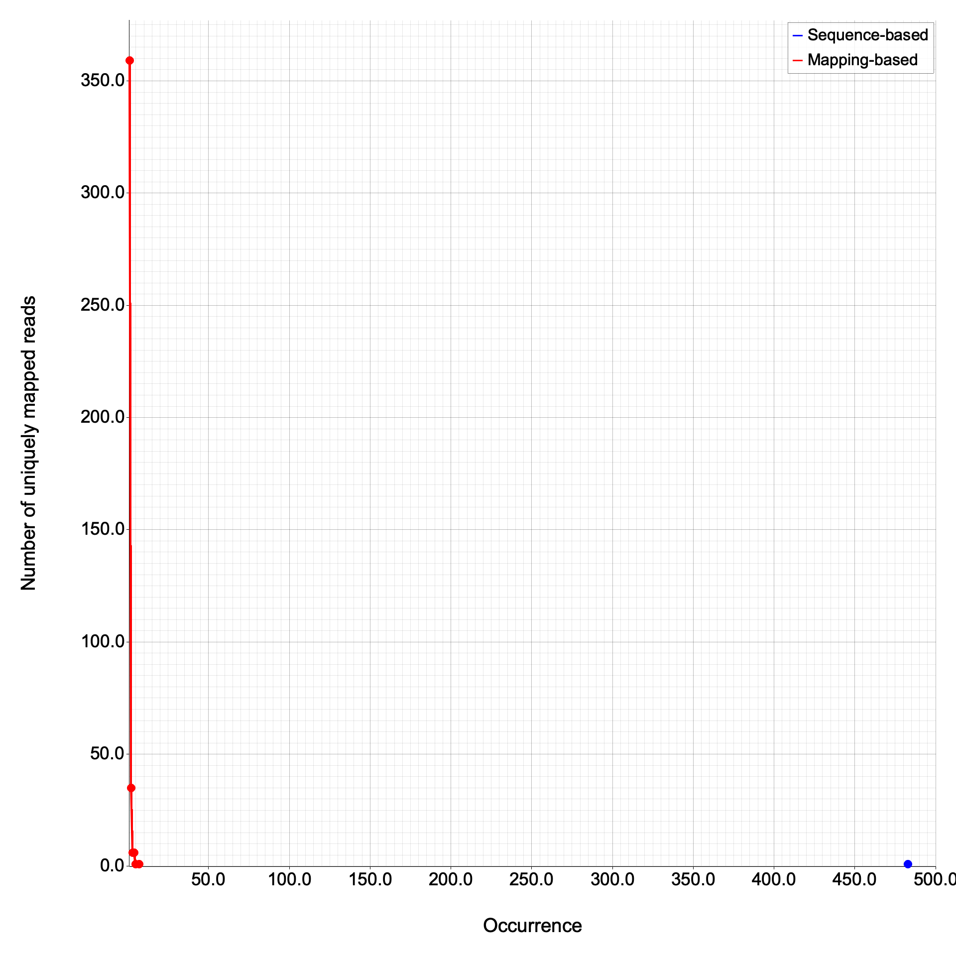
Position-based and sequence-based duplication rate histograms.
| File | Description |
|---|---|
{stem}.pos.DupRate.xls | Position-based duplication histogram (TSV: Occurrence, UniqReadNumber, ReadNumber) |
{stem}.seq.DupRate.xls | Sequence-based duplication histogram (TSV: Occurrence, UniqReadNumber, ReadNumber) |
{stem}.DupRate_plot.png | Duplication rate plot (PNG) |
{stem}.DupRate_plot.svg | Duplication rate plot (SVG) |
Each TSV file is a tab-separated table where each row represents a duplication level (number of times a read was seen). The columns are:
Position-based deduplication groups reads by alignment position (chromosome, start, CIGAR-derived exon blocks). Sequence-based deduplication groups reads by the actual read sequence.
The duplication rate plot shows two curves: sequence-based (blue) and position-based (red) duplication. The x-axis shows the occurrence count (capped at 500) and the y-axis shows the number of reads at each duplication level. Most reads should appear at low occurrence counts; a long tail indicates high duplication.
Duplication rate
Classification of reads across genomic feature types.
| File | Description |
|---|---|
{stem}.read_distribution.txt | Tabular report with total reads, total tags, and per-region breakdown |
The output includes:
Splice junction classification against a reference gene model.
| File | Description |
|---|---|
{stem}.junction.xls | TSV with all observed junctions: chrom, intron_start(0-based), intron_end(1-based), read_count, annotation_status |
{stem}.junction.bed | BED12 file with color-coded junctions (red = known, green = partial novel, blue = complete novel) |
{stem}.junction_plot.r | R script for generating splice event and junction pie charts |
{stem}.splice_events.png | Splice events pie chart (PNG) |
{stem}.splice_events.svg | Splice events pie chart (SVG) |
{stem}.splice_junction.png | Splice junctions pie chart (PNG) |
{stem}.splice_junction.svg | Splice junctions pie chart (SVG) |
{stem}.junction_annotation.txt | Summary: total/known/partial novel/complete novel event and junction counts |
Junctions are classified by comparing splice sites (CIGAR N-operations) against the reference BED12 gene model:
Two pie charts are generated, one for splice events (reads) and one for splice junctions (unique splice sites). Each chart shows the proportion of known (blue), partial novel (red), and complete novel (green) splicing.
Splice events

Splice junctions
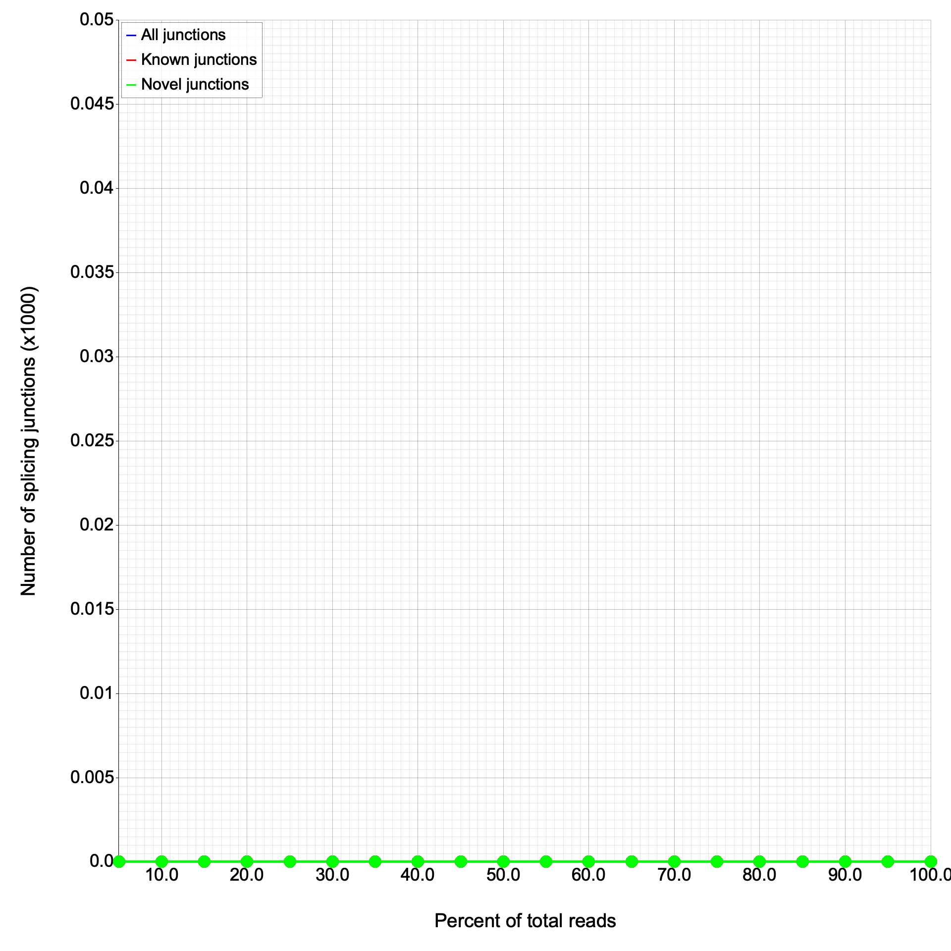
Splice junction discovery rate at increasing sequencing depths.
| File | Description |
|---|---|
{stem}.junctionSaturation_plot.r | R script for saturation curve plots |
{stem}.junctionSaturation_plot.png | Junction saturation plot (PNG) |
{stem}.junctionSaturation_plot.svg | Junction saturation plot (SVG) |
{stem}.junctionSaturation_summary.txt | TSV: percent_of_reads, known_junctions, novel_junctions, all_junctions |
The tool subsamples reads at configurable percentages (default: 5%, 10%, …, 100%) and counts how many unique known and novel junctions are detected at each level. This reveals whether sequencing depth is sufficient for comprehensive junction detection. A saturated library will show a plateau in the curve; an unsaturated library will show continuing growth.
The junction saturation plot shows three lines: all junctions (blue), known junctions (red), and novel junctions (green). The x-axis is the percentage of total reads used and the y-axis is the number of splice junctions detected (in thousands). A plateau in the curves indicates saturation.
Junction saturation
Fragment inner distance for paired-end RNA-seq libraries.
| File | Description |
|---|---|
{stem}.inner_distance.txt | Per-pair detail: readpair_name, inner_distance, classification |
{stem}.inner_distance_freq.txt | Histogram: lower_bound, upper_bound, count |
{stem}.inner_distance_plot.r | R script for histogram and density plot |
{stem}.inner_distance_plot.png | Inner distance histogram with density overlay (PNG) |
{stem}.inner_distance_plot.svg | Inner distance histogram with density overlay (SVG) |
{stem}.inner_distance_summary.txt | Summary counts by pair classification |
The inner distance is defined as the gap between the end of read 1 and the start of read 2 on the mRNA transcript. Negative values indicate read overlap. Pairs are classified as:
The histogram bins are configurable via --inner-distance-lower-bound,
--inner-distance-upper-bound, and --inner-distance-step (defaults: -250 to 250, step 5).
The inner distance plot is a histogram showing the distribution of fragment inner distances, with a Gaussian density curve (red) overlaid. The title displays the mean and standard deviation. The distribution should be approximately normal for a well-prepared library.
Inner distance

Measures transcript integrity via Shannon entropy of read coverage uniformity.
A reimplementation of RSeQC’s tin.py tool. For full details, see the
dedicated TIN & Gene Body Coverage documentation page.
| File | Description |
|---|---|
{stem}.tin.xls | Per-gene TIN scores (TSV: geneID, chrom, tx_start, tx_end, TIN) |
{stem}.summary.txt | Summary statistics: mean, median, and standard deviation of TIN scores |
TIN scores range from 0 (completely degraded) to 100 (perfectly uniform coverage). The tool uses the longest transcript per gene and samples equally-spaced positions within exonic regions.
All output files are designed to be drop-in replacements for the corresponding RSeQC Python tool output. File formats, column names, and numeric precision match the Python originals to facilitate migration from RSeQC to RustQC without downstream pipeline changes.
RustQC also generates the R scripts that RSeQC produces (for junction_annotation, junction_saturation, and inner_distance), maintaining full compatibility. However, unlike RSeQC, RustQC generates the plots directly as PNG and SVG files — there is no need to run the R scripts separately.